Getting back into NumPy, Day 6, 7, and 8

I had to prioritize some other stuff, so even though I actually wrote some code, I didn’t manage to write about it. Anyhow…

I haven’t gotten to implementing the actual algorithm yet, hopefully I’ll do that tomorrow, or over easter. What I have been doing is two things: visualization and refactoring. Let’s get the boring part (refactoring) out of the way first, and then we’ll look at the visualization and the problems I had with it.

The refactoring was very unglamourous. I put the problem setup into its own class, and wrote some class functions to plot it, apply the aperture, and so on and so on. This shorted the main program down to the following:

import ProblemSetup
ps = ProblemSetup.ProblemSetup()

Here, ProblemSetup is the class containing, you guessed it, the problem setup.

The class looks like follows. For clarity, I’ve removed almost all code, since you can find the details in the previous blog posts. What I want to show here is the structure.

import numpy as np
import matplotlib.pyplot as plt
import dcolor
class ProblemSetup:
    def __init__(self, n=100, aperture_form="circle", aperture_size=10, plot=True):
        self._n = n
        self._aperture_form = "circle"
        self._aperture_size = 10
        self._plot = True
        # Set up for plotting of dcolor image
        self.dc = dcolor.dcolor()
        ## Create aperture
        ... see earlier blog post ...
        
        self._start_guess = np.random.randn(n, n)
        if self._plot:
            self.plot_setup()
def apply_aperture(self, matrix):
    return np.multiply(matrix, self._aperture)
def apply_fft(self, matrix):
    return np.fft.fftshift(np.fft.fft2(matrix))
def plot_setup(self):
    ... plotting stuff ...

Not that fancy, but it works.

But now to the nice part! The visualization. So far I’ve plotted the magnitude of the FFT, but what we really is after is the phase of the wave. It is called a Phase Reconstruction Problem after all.

There is a way to nicely plot complex valued functions and matrices, and that is to use Domain Coloring. This produces colorful and informative images, so I thought I’d give it a go! And I found a python library for this as well, so what can go wrong?

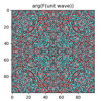
Well, apparently a lot, and what’s even worse: I haven’t solved the problem yet. I made some small changes to the code in the dcolor library to make it accept complex valued matrices, and then I plotted, hoping for a beautiful plot of the wave.

And I got one! Kind of…

It’s not supposed to look like that. For some reason, the phase is changing strongly from one pixel to another.

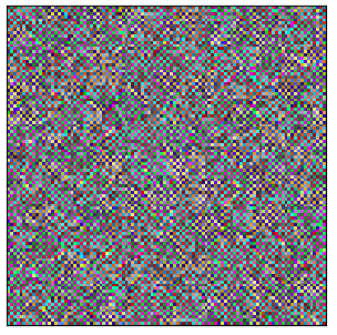
The same happens with the random start guess.

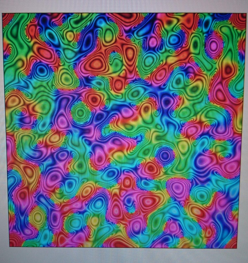
I tried a lot of things, nothing yielding anything useful. Until I resized the image back and forth. And suddenly!

To me, it seems that some kind of aliasing is happening. At this point in time, I am not quite sure if it is an aliasing problem, or if aliasing solved the problem. I’ll have to take a look at this during the upcoming days. This plot isn’t necessary for the algorithm, it is more a nice-to-have.

Anyhow, I’ll continue tomorrow, and hopefully the aliasing problem will have solved itself by then…