Getting back into NumPy, Day 4

(I didn’t do anything yesterday. Schande über mein Haupt as you say in German)

I have too little data to continue with the keystroke analysis, so in order to generate data I’m switching subjects. I decided to take on the subject for my master’s thesis: alternating projections.

The idea is as follows. You have a problem, where you have a vector y (e.g. a measurement), and you know that F(x) = y. Now you want to find the vector x. You know some conditions that x has to fulfill, and these conditions can be described as two or more sets. An example of such a set would be that x needs to lie within a circle.

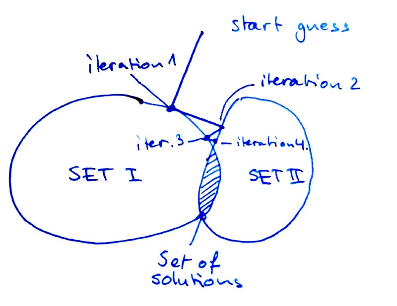
If x is a solution, then it must be a member of all of these sets, so x must lie in the intersection. And what you can do is to start with a guess x₀, project this initial guess onto one of the sets (and get x₁), project x₁ to the second set to get x₂, and so on. See the image below for a badly drawn explanation.

Rough sketch on how alternating projections work. In step 1, project the start guess onto set 1. In step 2, project the projection onto set 2, and so on until convergence is reached. In this particular case we’ll consider a complex wave front that passes through an aperture and the amplitude refractive pattern is measured. We want to compute the phase of the complex wave. In short, we have a phase reconstruction problem.

To keep things simple we will consider the far field, which means that our operator F is the Fourier transform (You can read more about why this is the case here. To be honest, I’m a bit fuzzy on the details).

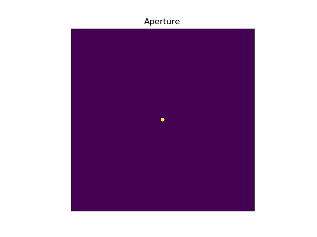
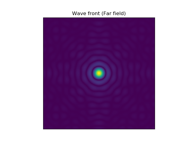
Today’s task is to create a matrix describing the aperture (in our case a circular aperture), and computing a unit wave’s FFT.

The code for this can be found below. It was surprisingly easy and the only tricky part was to make a circular aperture. Stackoverflow to the rescue! Using a mask, this is a one-liner.

import numpy as np
import matplotlib.pyplot as plt
# Settings
n = 1000 # Size of matrix
aperture_radius = 10 # Size of aperture radius
plot_aperture = True
plot_fft = True
# Counter for figures to be able to show several of them
figure_counter = 0
## Create aperture
x = np.arange(0,n)
y = np.arange(0,n)
aperture = np.zeros([n, n])
# Center of aperture
cx = int(n/2)
cy = int(n/2)
# Create circular aperture mask of given radius
aperture_mask = (x[np.newaxis,:]-cx)**2 + (y[:,np.newaxis]-cy)**2 < aperture_radius**2
aperture[aperture_mask] = 1
# ... Plotting stuff
## FFT of aperture
# FFT shift to make image pretty
fft = np.fft.fftshift(np.fft.fft2(aperture))
# Get intensity of wave front
abs_fft = abs(fft)
# ... Plotting stuff
plt.show()

The two pictures are… well, not pretty, but at least they look as we expect.

In my next post I’ll describe the sets that limits the wave front a bit more.